The way they are discussed for SAT and GRE exams usually doesn't give students a good intuition.
Examples
Most probabilities are not independent, which means they have some sort of correlation. (Examples...)(correlated-examples)
(start correlated-examples)
This US presidential election year, we have Trump as the Republican candidate and Hillary as the Democratic candidate. The chance that Hillary wins has a negative correlation with the chance that Trump wins, since knowing that one has won tells you that the other winning is less likely. Similarly, the chance that Hillary files an executive order has a positive correlation with the chance that Hillary wins the election, since knowing Hillary has become president tells you that filing an executive order is more likely.
(stop correlated-examples)
So, independent probabilities are not like those, but are instead entirely unrelated, with no correlation whatsoever. (Examples...)(independent-examples)
(start independent-examples)
The best examples often sound completely off the wall, like the chance of Trump winning the presidential election being independent with the chance you will eat soup this week. Another could be the chance that you roll an even number on a die being independent with the chance that I find a penny on the ground this month.
(stop independent-examples)
Intersection Probability
So now comes the interesting part. If you have two independent events \(U\) and \(V\), with probabilities \(P(U)\) and \(P(V)\), what's the chance of both occurring, [written \(P(U\cap V)\)?][(said "the probability of the intersection of U and V" or "P of U cap V")]
You may think that the independence of \(U\) and \(V\) means we know very little about how they are related, but it's actually the opposite: We know they are completely unrelated. This unrelatedness means there must be a (fixed value for \(P(U\cap V),\)!Fixed Intersection.)(fixed-intersection) and further, it gives us (a symmetry!A symmetry.)(independent-symmetry).
(start fixed-intersection)
Recall that for our pair of independent events \(U\) and \(V,\) there can be no positive or negative correlation. Each of the chances \(P(U)\) and \(P(V)\) are fixed, and there must be some chance \(P(U\cap V)\) that they have together. If \(P(U\cap V)\) were any larger, then \(U\) and \(V\) would have a positive correlation, and if \(P(U\cap V)\) were any smaller, then \(U\) and \(V\) would have a negative correlation. So, there must be some fixed value for \(P(U\cap V)\) when there is no correlation at all.
(stop fixed-intersection)
(start independent-symmetry)
If \(U\) and \(V\) are actually independent events, then knowing that one event has happened should not affect the probability of the other. In particular, if we look at only situations where \(U\) occurred, we should get the same probabilities for \(V\) occurring within those as within all possible situations. <!TODO: link to page about general definition of symmetry with "If it's unclear why I call this property a symmetry, click here.">
(stop independent-symmetry)
Now we can use that symmetry to find \(P(U\cap V)\). Here are two different but equally good ways to explain this step. (In terms of random sampling...)(random-sampling) (With a diagram...)(with-a-diagram)
(start random-sampling)
First note that with a total sample size of \(N\), if the sample size is large enough, the number of samples where \(U\) occurs should be about \(N\cdot P(U).\) If \(U\) is a set of possibilities chosen randomly as far as \(V\) cares, and if the sample size \(N\cdot P(U)\) of samples where \(U\) occurs is large enough, then the symmetry of independence says the number of those samples where \(V\) occurs should be about \((N\cdot P(U))\cdot P(V).\) Since these are the total number of samples where \(U\) and \(V\) both occur, it must be about equal to \(N\cdot P(U\cap V)\). After you divide both by the total sample size \(N\), you get the result \(P(U\cap V) = P(U)\cdot P(V).\) (All statistics assumes \(N\) is large enough to make the differences small enough to not care.)
(stop random-sampling)
(start with-a-diagram)
Consider the symmetry of independence with a Venn diagram: (What is this?)(what-venn-diagram) (Why we can use it?)(why-venn-diagram)
(start what-venn-diagram)
This diagram is meant to show geometrically how every situation is in one of the following cases:
- \(U\) happened, but not \(V\) (blue)
- \(V\) happened, but not \(U\) (red)
- \(U\) and \(V\) both happened (purple-ish)
- neither \(U\) nor \(V\) happened (green)
(stop what-venn-diagram)
(start why-venn-diagram)
We know all possible situations are illustrated because for each of the events, they must either happen or not happen. (This is the same reasoning that tells us that \(P(U)\) and \(P(\operatorname{not}U)\) add up to \(1\).)
(stop why-venn-diagram)
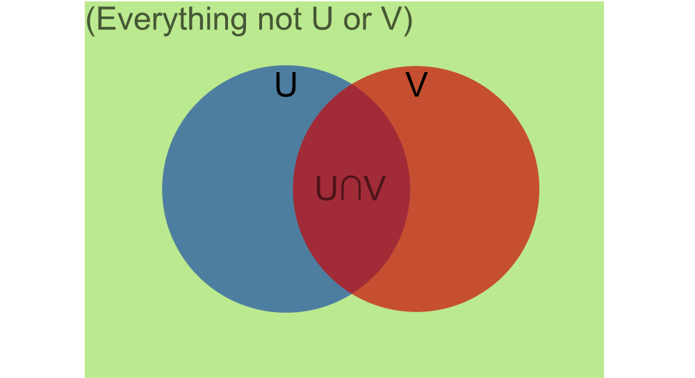
The symmetry says that \(P(V)\), how much of the whole rectangle is covered by the red \(V\) circle, needs to be equal to how much of the blue \(U\) circle is covered by the purple intersection. Since \(P(U)\) is how much of the whole rectangle is covered by the blue \(U\) circle, that means multiplying the two probabilities should give the probability for the purple intersection:
\[
\begin{aligned}
&P(U)\cdot P(V) \\
&= \frac{\text{blue circle}}{\text{green rectangle}}
\cdot\frac{\text{purple intersection}}{\text{blue circle}} \\
&=\frac{\text{purple intersection}}{\text{green rectangle}} \\
&= P(U\cap V)
\end{aligned}
\]
(stop with-a-diagram)
A Better Diagram
Now that we know what \(P(U\cap V)\) is, we can actually reduce all problems with independent probabilities to geometric ones using (a better diagram!Better diagram.)(better-diagram) than the generic Venn diagram in the last section.
(start better-diagram)
Since \(P(U\cap V)=P(U)\cdot P(V),\) it makes sense that we might want \(U\cap V\) to be represented by a rectangle with side lengths \(P(U)\) and \(P(V)\). If that rectangle were placed inside a shape with an area of \(1\) square unit, then the proportion of area covered by \(U\cap V\) would equal \(P(U\cap V).\) It just so happens that if you choose to put it inside a square with side length \(1,\) then this gives a full picture of the situation:
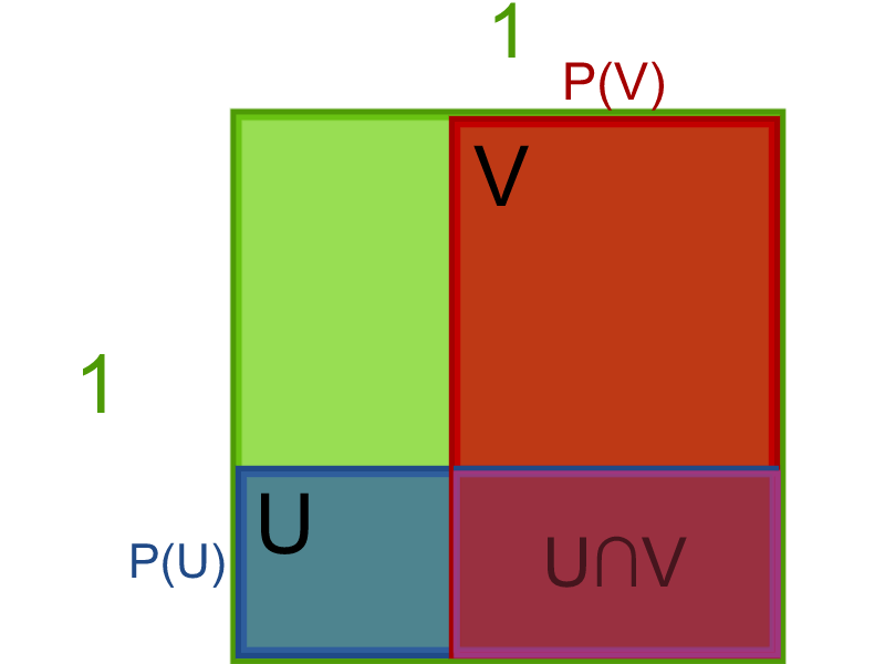
This works because it (meets all the conditions!Conditions.)(better-conditions). After drawing it, it (matches intuition!Intuition.)(better-intuition) about independent events. And it's a better diagram because you can (find all the probabilities geometrically!Geometric Probabilities.)(better-geometry).
(start better-conditions)
- The chance of a point in the square being in \(U\) is \(P(U).\)
- The chance of a point in the square being in \(V\) is \(P(V).\)
- The chance of a point in the square being in both is \(P(U)\cdot P(V).\)
(stop better-conditions)
(start better-intuition)
The intuition comes from measuring out the probabilities in independent dimensions. Think of it this way: If you choose a random point in the square, its \(x\)-coordinate tells you whether \(U\) happened, and its \(y\)-coordinate tells you whether \(V\) happened. Since independent variables told you each thing, knowing one doesn't affect the other. You can even extend this reasoning to three events, measuring out their probabilities as lengths on the edges of a cube.
(stop better-intuition)
(start better-geometry)
-
The chance of a point being in \(U\) or \(V\) is [\(P(U)+P(V)-P(U)\cdot P(V).\)][(found by adding the areas of \(U\) and \(V\) together and subtracting off the area of \(U\cap V\) since it was counted twice)]
-
The chance of a point being in \(U\) but not \(V\) is [\(P(U) - P(U)\cdot P(V)\)][(found by starting with the area of \(U\) and subtracting off the area of \(U\cap V\))] or [\(P(U)\cdot(1-P(V)).\)][(found by finding that the length from the top of the square to the top of \(U\) is \(1-P(V)\))] Similarly, the chance of a point being in \(V\) but not \(U\) is \(P(V)-P(U)\cdot P(V)=P(V)\cdot(1-P(U)).\)
-
The chance of a point not being in \(U\) or \(V\) is [\(1-P(U)-P(V)+P(U)\cdot P(V)\)][(found by starting with the whole square and subtracting off \(U\) and \(V,\) adding back \(U\cap V\) since it was subtracted twice)] or [\((1-P(U))\cdot(1-P(V)).\)][(found by finding the lengths from the top-left to the edges of \(U\) and \(V\) and multiplying them together)]
(stop better-geometry)
(stop better-diagram)